This is part 3 of a series on financial machine learning for people who know some Python and have never trained a model on financial data. Part 1 set out the vocabulary and the metrics. Part 2 built a dataset, broke it eight ways, and wrote the checks that caught the breaks. Its logistic regression was a measuring instrument: change the data, watch the score move.
This post makes that model the subject. We will train it, compare it with two simpler answers, decide what its probabilities mean, and use it to choose a review queue. Then we will freeze those decisions and open the test period.
The question I want to answer is small: when the model says 10%, does it mean 10%? A model can put the riskiest borrowers at the top of a list and still get that question badly wrong.
#A number between zero and one is not enough
Suppose one in ten borrowers with a particular set of features will default. An ordinary probability model should learn about 0.10 for that group.
Now tell the training loss to count each default nine times as heavily as each non-default. The same group contains ten default observations and ninety non-default observations. In the weighted loss those become ninety against ninety. The model's best answer is now 0.50.
Nothing is broken. It answered the question the loss asked.
That is the first trap in this post. A sigmoid makes an output fall between zero and one. It does not make a class-weighted output an estimate of the original event probability. We will see the effect on the same mortgage panel from part 2, then separate it from another problem: probabilities going stale when the population changes.
#The companion code
Everything below comes from
financial-ml-from-zero, part 3.
Keep part-03-baseline beside part-02-leakage. The new folder imports
the previous post's loader, labels, features, preprocessing, and checks.
There is no second implementation quietly changing the experiment.
The README covers environment setup. From part-03-baseline, run:
python ../part-02-leakage/make_synthetic_freddie.py --out data/synthetic --loans 12000 --seed 7
python run_baseline.py develop --data data/synthetic --out artifacts/baseline
python run_baseline.py evaluate --data data/synthetic --out artifacts/baseline
If you already generated the panel for part 2, skip the first command and point both later commands at that directory. Everything runs on a CPU. The development command writes the validation report and a frozen model. The evaluation command reads that model and writes the test report. It fits nothing.
Every measured result in this post comes from synthetic data. The
generator models a rise and fall in risk around 2009; its numbers are
not estimates of real mortgage performance. The small aggregate reports
are included in example-results, and the commands also write
calibration plots and individual test predictions with their loan IDs
and decision months.
#The contract, before the model
We are monitoring existing mortgages at the end of each reporting month. The population is reported, active loans currently less than 90 days past due. That includes loans one or two months behind; it is not restricted to borrowers paying on time. This is a behavioural risk model, using repayment history, rather than an application model deciding whether to grant a new loan.
The target is unchanged: did the loan reach 90 or more days past due, or end in a coded default, in the next twelve months? I will call that the default event below. It is the operational definition in this example, not a claim that every institution uses the same definition.
The ten features and the time windows are unchanged too:
| Split | Decision months | Last month its full label window needs | What it may decide |
|---|---|---|---|
| Train | Jun 2005–Dec 2007 | Dec 2008 | Preprocessing, model coefficients, class weight, benchmark probabilities |
| Validation | Jan–Dec 2009 | Dec 2010 | Which fitted model to use and the review threshold |
| Test | Jan–Dec 2011 | Dec 2012 | The final report |
The development command drops performance reports after December 2010 before it builds labels or features. By that date all of the validation year's twelve-month outcomes can be known. The test command uses reports through December 2012 to observe the test outcomes.
This is still the simplified timing contract from part 2: a monthly report is available at its month end. Actual reporting delays would move the usable dates. The wrapper also stops on missing reports, unknown delinquency status, or loans that stop reporting early without a closure code. An unobserved outcome is not a safe negative just because the dataset as a whole reaches December 2012.
There is one row per loan-month, not one row per independent borrower. A loan can appear in several months and in more than one split. That fits later monitoring of an existing portfolio. It does not establish performance on entirely unseen borrowers, and it does not justify confidence intervals that pretend every row is independent.
#Two answers the model has to beat
#Give everyone the training default rate
The first benchmark predicts the same probability for every row:
train_rate = float(y_train.double().mean())
constant = np.full(len(valid), train_rate)
On this panel that is about 2.92%. There are no features, no training loop, and no ranking power. Its ROC-AUC is 0.5. Its average precision equals the event rate of the period being evaluated, because all rows have the same score.
It is still a serious benchmark for probability quality. When events are rare, an elaborate model that overpredicts them can lose to a constant on Brier score or log loss. If that happens, report it.
The value predicted comes from training. Filling every test row with the test default rate would use the answers to construct the benchmark.
#Use only how far behind the borrower already is
The second benchmark has three groups: current, one month behind, and two months behind. For each group, estimate its twelve-month event rate in training. Smooth it with twenty extra observations at the overall training rate so a small group does not produce an extreme probability:
groups = train.groupby("dq_status_now")[LABEL].agg(["sum", "count"])
rates = (groups["sum"] + 20 * train_rate) / (groups["count"] + 20)
Twenty is fixed for the example, not selected on the test set. Each validation or test row receives its group's training probability.
Part 2 already showed that current delinquency was the strongest single feature. This benchmark makes that observation operational. A ten-feature model should earn its extra moving parts against a rule a colleague can explain in one sentence.
#Logistic regression, one line at a time
The model takes the ten standardised features, multiplies each by a learned weight, and adds a bias:
z = w1*x1 + w2*x2 + ... + w10*x10 + b
p = sigmoid(z) = 1 / (1 + exp(-z))
The first number, z, is the logit. For an ordinary probability
model it represents log-odds: a probability of 0.10 has odds of one to
nine and log-odds of about −2.20. The sigmoid converts back to a
probability.
In PyTorch the model is almost the same size as the equation:
class LogisticRegression(nn.Module):
    def __init__(self, n_features: int):
        super().__init__()
        self.linear = nn.Linear(n_features, 1, dtype=torch.float64)
        nn.init.zeros_(self.linear.weight)
        nn.init.zeros_(self.linear.bias)

    def forward(self, x):
        return self.linear(x.to(torch.float64)).squeeze(-1)
It returns logits, not probabilities. The loss will handle the sigmoid. There are eleven learned numbers: ten weights and one bias. There is no hidden layer, dropout, or architecture search. The tensors come from the same training-only median filling and scaling as part 2; the fit uses double precision to make convergence checks more stable.
#What the loss asks for
For a binary outcome, ordinary binary cross-entropy penalises the model for giving low probability to the outcome that actually happened:
loss = -[y * log(p) + (1 - y) * log(1 - p)]When y is one, only the first term remains. Predicting 0.01 for an
event that happens costs much more than predicting 0.60. When y is
zero, the second term does the corresponding job for a non-event.
Use BCEWithLogitsLoss, which combines the sigmoid and the loss in a
numerically stable calculation. Do not apply a sigmoid first and pass
the resulting probabilities to this loss. Its input is the logit.
That input contract is documented in
PyTorch's loss reference.
#Fit far enough that the comparison means something
Part 2 found that a short Adam run could make a harmless scaling change look like a leakage effect. Here the dataset and model are small enough to use full-batch L-BFGS, an optimiser that uses gradient history to choose its steps. The whole training window fits in memory.
Its slightly unusual feature is a closure: a function it can call again to calculate the loss and gradients at a candidate set of weights. The core is:
def closure():
    optimiser.zero_grad()
    loss = loss_fn(model(x_train), y_train.double())
    loss.backward()
    return loss

optimiser.step(closure)
zero_grad clears the previous gradients. backward calculates how
the loss changes with each weight. The optimiser uses those changes
to move the weights. It may call the closure several times per step.
The companion allows up to 500 iterations, uses a line search, then
recomputes the largest absolute gradient. It stops with an error if
that gradient exceeds 1e-5. That is a convergence check, not a
guarantee that the model is correctly specified. We fit without a
regularisation penalty here so the loss comparison stays easy to see.
#Class imbalance: what weighting changes
Only about 2.92% of training rows have a positive label. A common response is to give positives a weight equal to the number of negatives divided by the number of positives:
positive_weight = float((len(y_train) - y_train.sum()) / y_train.sum())
loss_fn = nn.BCEWithLogitsLoss(
    pos_weight=torch.tensor(positive_weight, dtype=torch.float64)
)
That is about 33 here. The calculation uses training labels only.
The ordinary model is the same fit with positive_weight=1.0.
Weighting changes the objective. A missed positive now costs more in training. It can be useful when recall matters, but it is not a free repair for rare events, and an unweighted probability loss is not invalid merely because one class is rare.
Write p for the original event probability, w for the positive
weight, and q for the best answer under weighted loss. Minimising
that loss at a fixed set of features gives:
q = w*p / (1 - p + w*p)
logit(q) = logit(p) + log(w)
That is why 10% becomes 50% when the weight is nine. The weighted answer has different odds.
We can remove that known shift from the weighted model's logits:
corrected_probability = torch.sigmoid(weighted_logits - math.log(positive_weight))The report calls this weighted_corrected. Subtracting the same
constant from every logit leaves the ordering unchanged. Its average
precision and ROC-AUC therefore match the raw weighted model's scores.
Its probability metrics can be very different.
There are two limits to that correction. The formula describes the ideal weighted optimum; a finite linear model may not represent the true relationship, and weighting can change fitted slopes as well as the intercept. More importantly, removing the training weight says nothing about how risk changes between training and deployment. An odds correction is not a certificate of calibration.
#The validation report
The companion reports five rows: constant probability, delinquency only, unweighted logistic regression, raw weighted logistic regression, and weighted logistic regression after the odds correction.
Validation has 81,869 rows and 4,356 positive labels: an event rate of 5.32%, against 2.92% in training.
| Model | Mean prediction | AP ↑ | ROC-AUC ↑ | Brier ↓ | Log loss ↓ |
|---|---|---|---|---|---|
| Constant training rate | 2.92% | 0.0532 | 0.5000 | 0.05095 | 0.21608 |
| Delinquency only | 3.80% | 0.2155 | 0.6376 | 0.04341 | 0.18255 |
| Unweighted logistic | 4.48% | 0.3094 | 0.7832 | 0.04291 | 0.17226 |
| Weighted, raw | 42.43% | 0.3130 | 0.7844 | 0.21385 | 0.63907 |
| Weighted, odds corrected | 4.84% | 0.3130 | 0.7844 | 0.04321 | 0.17408 |
There is a naming detail worth fixing before more posts build on it.
Part 2 called its precision-recall metric PR-AUC, but the implementation
was average_precision_score. Here I use its precise name,
average precision (AP). It adds precision values weighted by the
increase in recall; it is not the trapezoidal area under an
interpolated curve. The
scikit-learn reference
explains the distinction. These AP results are comparable with the
implementation in part 2.
AP and ROC-AUC ask about ranking. Brier score and log loss ask about probability quality. Lower is better for the latter two. Brier is the mean squared difference between the probability and the zero-or-one outcome. Log loss penalises confident wrong answers more sharply.
Neither is a pure calibration metric. A change in discrimination or in the event rate can change them too. That is why the next thing to read is a calibration curve, with its counts alongside it, rather than declaring a model calibrated because one loss went down.
The raw weighted model is the opening mistake made concrete. Its ranking is slightly better than the ordinary model's, but its mean prediction is 42.43% in a population with a 5.32% event rate. Its log loss is worse than predicting the training base rate for everyone.
The odds correction brings the mean down to 4.84% without changing the ranking. The ordinary model still has the lower log loss and Brier score. The AP difference, 0.3094 against 0.3130, is small; one validation year is not enough to establish that weighting reliably improves ranking.
The delinquency-only benchmark is worth noticing too. It gets much of the Brier improvement over the constant before we train anything with ten features. The full model adds more ranking power and improves log loss, but the simple answer was already doing useful work.
#Read the probabilities, not just the ranking
A reliability diagram, or calibration curve, groups predictions into probability bands. For each band it plots the average prediction against the fraction of rows where the event actually occurred. If rows given roughly 10% predictions have roughly a 10% event rate, that point sits near the diagonal.
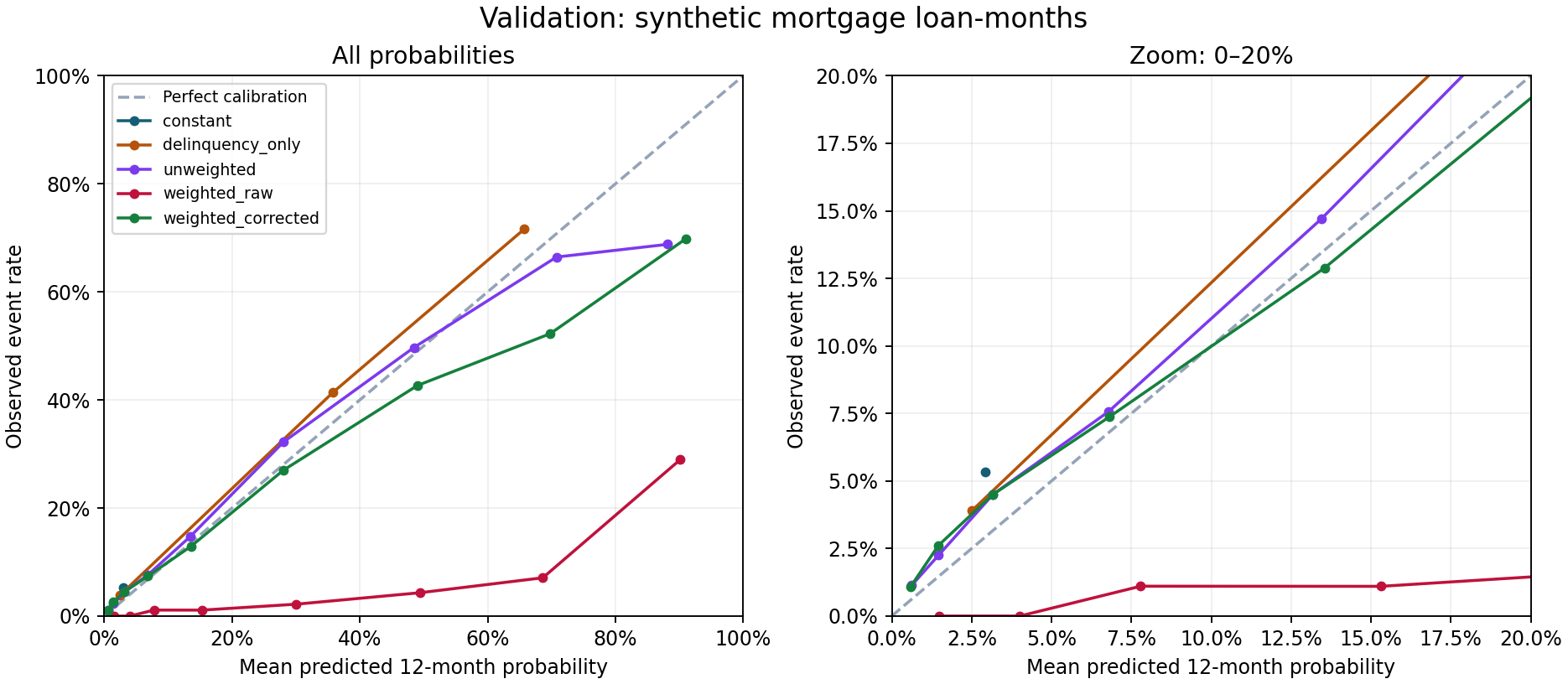
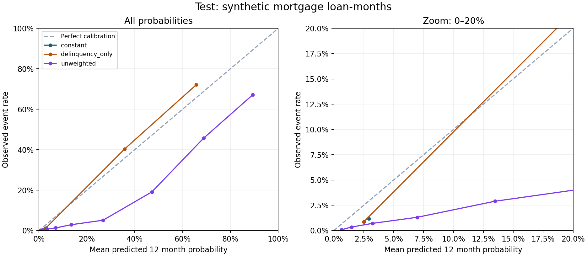
The bands are fixed before evaluation: 0–1%, 1–2%, 2–5%, 5–10%, 10–20%, then wider bands up to 100%. The saved CSV includes the number of rows and events in every occupied band. Empty bands are omitted; they are not evidence of zero observed risk.
A point above the diagonal means the model underestimated the observed event rate in that band. A point below it means it overestimated. A high-probability band containing a handful of rows deserves less confidence than one containing thousands, and even thousands of loan-months do not mean thousands of independent loans.
There is a separate technique called post-hoc calibration: fit a mapping from a model's scores to probabilities on held-out labelled data. We do not fit one here. The validation year already chooses the model and review threshold; fitting a calibrator there and showing its fit on that same year as independent evidence would be misleading. A separate calibration window, with mature outcomes and a later evaluation window, belongs in the walk-forward design of part 4. The scikit-learn calibration guide describes why the calibrator needs data independent of the model fit.
#Turn a probability into a review decision
A probability and a decision are different objects. Nothing about a 0.5 threshold is automatically right for rare defaults.
For this example, imagine a monitoring team that can review at most 10% of the validation period's loan-months. That is a teaching budget, not a claim about a real team's staffing or the financial value of review. We choose the lowest score threshold that fits that budget, keeping equal scores together.
values, counts = np.unique(p_valid, return_counts=True)
values, counts = values[::-1], counts[::-1]
allowed = np.cumsum(counts) <= math.floor(len(p_valid) * 0.10)
threshold = values[allowed][-1] if allowed.any() else np.nextafter(1.0, 2.0)
The final line handles a useful edge case. A constant model ties every row. A probability threshold can review everybody or nobody; it cannot pick the riskiest 10%. We choose nobody instead of breaking ties with an arbitrary row order. A random queue would be a different policy and should be named as such.
The learned model's threshold is frozen with its coefficients. When the test distribution changes, the share above that threshold is allowed to change. Selecting the top 10% afresh each month would be a valid capacity policy, but it is a different policy from the fixed cutoff evaluated here. This example uses one pooled validation budget; it does not guarantee a monthly staffing limit.
Review also does not mean decline a loan or prevent a default. We can measure who entered the queue and what later happened. These labels do not tell us what would have happened under an intervention.
#Freeze the choices, then use the test split
The selection rule is written into the development command: choose the lower validation log loss of unweighted and weighted_corrected. The raw weighted output stays in the report to show the probability trap; it is not a candidate PD estimate. Both simpler benchmarks stay in the final report regardless of which logistic model wins.
The rule selects the unweighted model, with validation log loss 0.17226 against 0.17408 for the corrected weighted model. Its review threshold is 0.078845, or about 7.88%. That number comes from the validation score distribution and the stated review budget; it is not a universal credit-risk cutoff.
The command saves frozen.json: feature order, training medians and
scales, selected weights and bias, any logit correction, benchmark
probabilities, review thresholds, package versions, and hashes of the
code and source files. The evaluation command checks those hashes and
loads the saved numbers. It does not choose another model, fit another
scaler, or move the threshold.
It also creates test-started.json before building the test examples
and refuses to evaluate that run again. Development refuses to
overwrite a frozen run. These guards catch an accidental rerun; they
cannot stop someone deleting a file or making a new output directory.
Once the result is visible, another design needs another genuinely
unseen evaluation period.
One disclosure matters: part 2 already printed the test split's size and base rate. This is not a claim of a completely blind research benchmark. The rule we can enforce here is narrower: no test-period model comparison, fitting, calibration, or threshold selection.
Here is the single final evaluation, on January–December 2011:
Test has 84,656 rows and 987 positive labels: an event rate of 1.17%.
| Model | Mean prediction | AP ↑ | ROC-AUC ↑ | Brier ↓ | Log loss ↓ |
|---|---|---|---|---|---|
| Constant training rate | 2.92% | 0.0117 | 0.5000 | 0.01183 | 0.07048 |
| Delinquency only | 2.76% | 0.1661 | 0.6263 | 0.01020 | 0.06078 |
| Frozen unweighted logistic | 4.83% | 0.2026 | 0.8057 | 0.01339 | 0.07458 |
The model still ranks risk better than either benchmark. Its ROC-AUC is actually higher than it was on validation. But it predicts an average 4.83% against an observed 1.17%, and loses to both benchmarks on Brier score and log loss.
That is the second trap. Removing class weights did not make the probabilities portable across time. The training relationship between the ten features and risk does not describe this later period well enough. The simulation's crisis has passed; the model's predictions have not followed the event rate down. The calibration curve makes the mismatch visible.
The drop in AP from 0.3094 to 0.2026 should not be read in isolation: the event rate also fell from 5.32% to 1.17%. Compare models within each period and keep its base rate visible. A change in AP between populations mixes changes in prevalence with changes in ranking.
I would keep this model as a reproducible development baseline. I would not use its test-period probabilities as reliable risk estimates. The result suggests investigating time drift and calibration in the next experiment. It does not authorise fitting a correction to the 987 test positives and presenting the corrected result as another independent test.
The same frozen review rules produce:
| Policy | Reviewed rows | Share reviewed | Positive rows caught | False alerts | Positive rows missed | Precision | Recall |
|---|---|---|---|---|---|---|---|
| Constant, ties kept together | 0 | 0.00% | 0 | 0 | 987 | — | 0.00% |
| Delinquency only | 489 | 0.58% | 252 | 237 | 735 | 51.53% | 25.53% |
| Frozen logistic cutoff | 12,751 | 15.06% | 554 | 12,197 | 433 | 4.34% | 56.13% |
The counts are positive loan-month labels, not distinct defaulted loans. Several monthly predictions can refer to the same future default. Precision is the share of reviewed rows with a positive label; recall is the share of all positive rows sent for review. Precision is undefined for an empty queue, which the report leaves blank rather than presenting as a measured zero.
The logistic policy catches 554 of the 987 positive rows, with about 22 false alerts for each positive caught. It sends 15.06% of rows for review, even though its threshold covered at most 10% on validation. A frozen score cutoff does not freeze the queue size.
The delinquency rule produces a much smaller, more concentrated queue and misses more positive rows. These are not equal-workload policies: its three tied score groups cannot fill an arbitrary 10% budget without a separate tie-breaking rule. The table shows the operational trade-off; it does not establish which model is best at an identical review capacity.
#Checks that make this a baseline worth keeping
The companion includes a small test suite:
python -m unittest -v test_baselineIt checks the contracts that are easy to get subtly wrong. On an intercept-only dataset with a 10% event rate, ordinary training must learn 0.10, weight-nine training must learn 0.50, and the odds correction must return 0.10. The correction must preserve ranking. Calibration bands must retain predictions exactly at zero and one. Equal scores must not silently overfill the review budget.
The most important check changes every delinquency observation after the development cutoff and rebuilds the development rows. They must be identical. Another verifies that an existing evaluation marker stops the command before it loads test rows.
Those checks sit beside part 2's assertions about panel ordering, monthly calendars and gaps between split windows. A favourable score does not replace any of them.
#What is next
We have one training period, one validation period, and one test period. That is enough to finish a baseline. It is not enough to tell us whether its behaviour is stable through several regimes.
Part 4 is purged walk-forward validation: repeatedly move the training and evaluation windows forward, remove training examples whose label windows overlap evaluation, and make the role of an embargo explicit. It is also where we can give calibration its own proper place in time instead of asking one validation year to do every job.
#Summary to save
- Write down the population, decision time, event definition and horizon before training. A probability without those is incomplete.
- Keep a training-rate constant and a simple domain benchmark in the report. More features have to earn their place.
- Pass logits to
BCEWithLogitsLoss. Apply sigmoid when you need probabilities, not before that loss. - Positive-class weighting changes the probability target. Removing its log-odds shift does not repair model misspecification or time drift.
- Report ranking and probability quality separately. Read the calibration curve with the bin counts, not just one aggregate loss.
- Choose the decision policy on validation and say how ties work. A fixed threshold and a fixed queue size answer different questions.
- Freeze the preprocessing, model, benchmarks and policy before test evaluation. Keep the disappointing numbers in the report too.
- Count loan-months honestly. Repeated observations are not independent borrowers, and a detected event is not a prevented loss.